Strand 1 — State-dependent Kelly fraction
OU pretesting; stochastic-\(\kappa_t\) estimation via the macro-enriched state equation; the regime-collapse early-warning system. In progress.
Research
Independent and collaborative research on portfolio allocation, stochastic modeling, machine learning methods in finance, and quantum algorithms for financial risk.
An independent, self-directed research project, currently in progress. It builds on the strategic asset-allocation literature — Merton (1971), Kim–Omberg (1996), Wachter (2002) — and on distributionally robust optimisation (Rujeerapaiboon et al., 2016).
The work develops a unified robust Kelly framework for pension-fund welfare when a predictive state variable — a bond yield, a valuation ratio (CAPE), or a risk premium — is mean-reverting with an unknown, time-varying mean-reversion speed \(\kappa_t\), while the traded asset price follows a geometric Brownian motion driven by that state variable. It nests Wachter (2002), Rujeerapaiboon et al. (2016), and standard CPPI as limiting cases.
Central question: how should a pension fund allocate capital over a long accumulation horizon when a predictive state variable is mean-reverting but mean reversion may fail, and the investor faces a hard welfare floor below which wealth must not fall with probability greater than \(\varepsilon\)?
My research is motivated by a broader question: how should long-horizon portfolios adapt when the market regime changes, particularly when the investor cannot afford to wait for a conventional recovery? This question became particularly compelling to me through the experience of Germany's Riester pension system. A saver entering the market around 2000 could have experienced a 73% decline in the DAX by March 2003, while recovery to previous highs took more than a decade. For a retirement investor, such a drawdown is fundamentally different from a temporary mark-to-market loss: the timing of the loss relative to the investor's horizon can permanently alter the opportunity set. At the same time, Riester's legal nominal capital guarantee, combined with the prolonged low-interest-rate environment after 2012, created strong incentives for providers to maintain very high bond allocations. The resulting problem was therefore not simply nominal capital loss, but prolonged compression of real returns.
Although Riester is a German pension product, the underlying problem is not uniquely German. It is a general portfolio-construction problem that becomes increasingly relevant as India's retirement savings ecosystem deepens and moves toward market-linked instruments. Indian investors are increasingly exposed to equity-market cycles through mutual funds, pension products and other long-term savings vehicles, while the transition from guaranteed to market-linked retirement products raises the importance of managing sequence-of-returns risk and regime dependence.
This motivates my research: rather than treating asset allocation as a static optimization problem, I explore whether portfolio construction should respond dynamically to the prevailing market regime and investor horizon. My framework combines regime identification through mean reversion speed estimation which is dynamic with time, Bayesian uncertainty quantification, and robust optimization under a welfare floor. The goal is to provide a principled approach to long-horizon portfolio allocation that is sensitive to regime changes and the investor's risk tolerance.
Riester provides the motivating historical example; the broader research question is applicable to any economy where long-term savings increasingly depend on market-linked portfolio decisions.
The predictive state variable \(X_t\) follows a stochastic Ornstein–Uhlenbeck process with a latent, time-varying speed; the asset price \(S_t\) need not mean-revert:
The speed \(\kappa_t\) itself evolves as a latent stochastic process driven by macro covariates \(Z_t\) — yield-curve slope, central-bank policy path, ISM / ifo PMI, ZEW / Michigan sentiment (selected by LASSO):
Observable macro data let the posterior \(p(\kappa_t \mid \mathcal{F}_t)\) shift in real time, giving an early-warning signal for regime collapse before it shows up in price data.
Strand 1 — Stochastic mean reversion and the state-dependent Kelly fraction. Under log-utility, the optimal risky weight can be decomposed into a myopic Kelly component and an intertemporal hedging component arising from predictable changes in investment opportunities:
Here, \(\kappa_t\) governs the speed of mean reversion in the investment-opportunity process. Because \(\kappa_t\) is latent, the portfolio responds to its posterior distribution conditional on the information set \(\mathcal{F}_t\), rather than treating the regime as directly observable. As the posterior shifts toward a low mean-reversion state, the contribution of the mean-reversion-based hedging component diminishes, causing the allocation to converge toward its myopic Kelly component when the model-implied limiting condition \(h(\kappa,\cdot)\to0\) is satisfied as \(\kappa\to0\). The resulting adjustment is endogenous: no exogenous stop-loss or discretionary regime override is required. A macro-enriched state equation for \(\kappa_t\) then provides an economically interpretable early-warning signal for deterioration in the persistence and mean-reversion structure of expected returns.
Strand 2 — Bayesian uncertainty quantification. Constructs the full posterior \(p(\kappa_t \mid \mathcal{F}_t)\) via MCMC / Hamiltonian Monte Carlo, variational inference, and a Gaussian Process posterior over the trajectory, then propagates it into the Kelly fraction with an explicit epistemic–aleatoric decomposition. Epistemic (parameter) uncertainty alone drives constraint tightening; the posterior variance calibrates the Wasserstein ambiguity radius endogenously:
When the data strongly identify \(\kappa_t\) the ambiguity set is small and the allocation stays close to classical Kelly; near a unit root or after a structural break it expands and the optimisation turns conservative.
Strand 3 — Downside-constrained robust Kelly. The Riester guarantee is a path-wise chance constraint, \(\mathbb{P}(W_t < \bar{W}) \le \varepsilon\) for all \(t \in [0,T]\), where \(\bar{W}\) is the nominal sum of contributions. A safe ambiguity set restricts the adversary to floor-respecting distributions, and the allocation interpolates between classical and robust Kelly so that exposure degrades gracefully as uncertainty grows:
As \(\operatorname{Var}(\kappa_t \mid \mathcal{F}_t)\) rises, \(\lambda_t \to 1\) and \(f_t^{*} \to 0\) continuously — matching the smooth collapse of mean reversion rather than reacting after the fact.
US estimation laboratory: 10-year Treasury yield
(FRED, 1962–2024), S&P 500 CAPE (Shiller, 1871–2024), 3-month
T-bill, ISM Manufacturing PMI, University of Michigan Sentiment.
German out-of-sample application: DAX Total Return
(1988–2024), 10-year Bund yield, ifo Business Climate, ZEW Economic
Sentiment, GDV Riester fund returns (2002–2024), German CPI — across
three structural-break episodes: the post-2000 equity crash, the
post-2008 zero-lower-bound environment, and the post-2012 ECB QE
regime.
I'm working through this in three connected strands. The current focus is the first: OU pretesting for the state variables and stochastic-\(\kappa_t\) estimation via the macro-enriched state equation, together with the regime-collapse early-warning signal.
OU pretesting; stochastic-\(\kappa_t\) estimation via the macro-enriched state equation; the regime-collapse early-warning system. In progress.
Full posterior inference (MCMC, variational inference, Gaussian Processes); epistemic–aleatoric decomposition; propagation into the hedging demand and Wasserstein-radius calibration. Planned.
Tractability of the unified minimax problem; robust optimisation with the welfare floor; backtesting across the German structural-break episodes. Planned.
The framework is expected to outperform benchmarks on welfare protection — lower floor-breach frequency and smaller expected shortfall below \(\bar{W}\) — while staying competitive on growth in normal regimes. The central empirical claim: explicitly accounting for posterior uncertainty over \(\kappa_t\), rather than treating mean-reversion speed as a known constant, substantially closes the welfare gap between the unconstrained Kelly-optimal allocation and the conservative, guarantee-bound strategies Riester providers currently use.
Sole-authored, written in a personal capacity. Presented as my final project for the Quantum Computing certification at IIT Delhi.
Expected loss (EL) of a credit portfolio driven by a latent systematic risk factor is normally estimated by Monte Carlo, whose sampling complexity is \(O(\varepsilon^{-2})\) for target error \(\varepsilon\). This paper recasts EL under a discretized latent-factor model as a quantum amplitude estimation problem, recovering the quadratic speedup to \(O(\varepsilon^{-1})\) oracle queries.
A single systematic factor \(Z \sim \mathcal{N}(\mu, \sigma^2)\) drives the conditional default probability, and the loss is \(L(Z) = \text{EAD} \cdot \text{LGD} \cdot \text{PD}(Z)\), with target \(\mathbb{E}[L] = \int L(z)\,\varphi_{\mu,\sigma}(z)\,dz\). Discretizing \(Z\) on an \(N = 2^{n}\) grid over \([\mu - 3\sigma,\, \mu + 3\sigma]\) with bin masses \(p_i\) gives
The discretized distribution is loaded into an \(n\)-qubit uncertainty state, and the normalized loss \(\tilde{L}(z_i) = L(z_i)/L_{\max}\) is written onto an ancilla qubit via controlled \(Y\)-rotations by angle \(2\arcsin\sqrt{\tilde{L}(z_i)}\):
Applying the state-preparation operator to \(|0\rangle^{\otimes n}|0\rangle\) makes the probability of measuring the ancilla in \(|1\rangle\) equal to \(a = \sum_i p_i\,\tilde{L}(z_i) \approx \mathbb{E}[\tilde{L}]\), so \(\mathbb{E}[L] = L_{\max}\, a\). The resulting state admits a two-subspace decomposition, and \(a\) is recovered either by quantum amplitude estimation (phase estimation on the Grover operator) or by a maximum-likelihood estimator from Grover-power measurements, \(\Pr(\text{ancilla} = 1 \mid m) = \sin^2\!\big((2m+1)\theta\big)\).
Both routes achieve \(O(\varepsilon^{-1})\) oracle-query complexity against the classical \(O(\varepsilon^{-2})\). A synthetic latent-factor study with \(\text{PD}(Z) = \Phi(\alpha Z + \beta)\) confirms the RMSE of the EL estimate scaling as \(O(N^{-1})\) for ideal quantum queries versus \(O(N^{-1/2})\) for classical Monte Carlo.
Ghosh, Arghya. Quantum Amplitude Estimation for Expected Loss Computation under a Discretized Latent-Factor Model (January 30, 2026). Available at SSRN: ssrn.com/abstract=6334018 · doi:10.2139/ssrn.6334018
A monitoring methodology I developed after several years working in model risk. It derives, from first principles, a variance-adjusted band for loss-given-default (LGD) model performance — one that adjusts for the changing effective sample size of each monitoring snapshot and carries an explicit systematic-risk floor.
An LGD model is monitored by comparing predicted LGD against realized LGD on resolved loans. However, the number and composition of resolved loans can vary substantially across monitoring windows. In some cohorts, only one or two loans may have resolved, even within an otherwise healthy portfolio. In such cases, the realized LGD can be heavily driven by the idiosyncratic outcome of a single loan and may therefore provide an unreliable estimate of the underlying portfolio LGD. A large "predicted vs. actual" gap in such a small cohort may consequently reflect sampling noise rather than genuine model deterioration, yet a fixed monitoring threshold could still classify it as a breach and unfairly penalize the model. Instead of reducing each snapshot to a single pass/fail test, this note builds an interval around the historical baseline error, scaled to the current snapshot's effective sample size, that can be recomputed and plotted at every refresh.
A cohort is the set of loans that default within a fixed horizon measured from the snapshot date — 9 quarters (9Q) for CCAR stress testing and 8 quarters (8Q) for CECL. Write \(DB_k\) for the default balance (exposure at default) of loan \(k\), and \(lgd_k\) for its realized loss rate.
The quantity actually monitored is the cumulative, portfolio-level LGD for that cohort: the cohort's total expected loss over the horizon divided by the cohort's total default balance over the same horizon — equivalently, a default-balance-weighted average of the loan-level loss rates:
Here \(\text{Cum EL}^{\,t}_{H}\) is the cohort's cumulative expected loss over the horizon \(H\), the weights are \(W_k := DB_k / \text{Total } DB_{H,t}\), and \(H = 9\text{Q}\) for CCAR or \(H = 8\text{Q}\) for CECL. So the object of interest is not an average of per-loan errors but a single cumulative loss ratio for the whole resolved cohort, with large exposures carrying proportionally more weight.
Loan-level errors follow the standard regression decomposition \(lgd_{\text{actual},k} = lgd_{\text{model},k} + \varepsilon_k\) with \(\varepsilon_k \sim D(0, \sigma^2)\). Since the cohort LGD above is the balance-weighted average \(\sum_k W_k\, lgd_k\), under independence its variance is
This effective (Kish-type) sample size is at most the loan count and shrinks as the cohort concentrates in a few large exposures — the natural way to measure how many independent, equally-weighted observations a concentrated balance-weighted portfolio is worth.
LGD outcomes on loans resolving in the same window are not fully independent: common macro shocks, collateral-market conditions, sector or geographic concentration, and servicer effects induce positive correlation. A variance-components model captures this parsimoniously:
where \(\sigma^2 / n_{\text{eff},t}\) is the diversifiable idiosyncratic component and \(\tau^2 \ge 0\) is the systematic, undiversifiable risk component — a common-shock variance that does not average out no matter how large or granular the cohort. Setting \(\tau^2 = 0\) recovers the pure-independence case; \(\tau^2 > 0\) stops the band from becoming unrealistically tight for large, well-diversified snapshots.
\((\sigma^2, \tau^2)\) are estimated jointly from the historical pairs \(\{(e_t, n_{\text{eff},t})\}_{t=1}^{T}\) — either by OLS of squared residuals on \(1/n_{\text{eff},t}\) (intercept \(\to \tau^2\), slope \(\to \sigma^2\), with a \(\max(0, \cdot)\) truncation), or by a normal variance-components maximum-likelihood estimator. The MLE is recommended for production use, with OLS as a transparent diagnostic and a source of starting values.
For the current snapshot — observed aggregate residual \(e_0\), effective sample size \(n_{\text{eff},0}\), historical baseline error \(\hat{\mu}\) — the standard error and \(k\)-sigma band are
Flag the snapshot when \(e_0\) falls outside the band, at two conventional tiers: \(k = 2\) (warning, \(\alpha \approx 5\%\)) and \(k = 3\) (action, \(\alpha \approx 0.3\%\)). The band is snapshot-conditional — it narrows and widens each quarter with cohort composition — and, unlike the pure-independence version, asymptotes to \(\hat{\mu} \pm k\hat{\tau}\) as the cohort grows rather than collapsing to zero width. The floor is estimated from data through \(\hat{\tau}^2\) rather than imposed as an ad hoc minimum width.
An implementation and adaptation of D-TIPO — Deep Time-Inconsistent Portfolio Optimization with stocks and options (Andersson & Oosterlee, 2023) — to Indian equities. The finding: a small, statically-held option overlay materially raises the utility of the terminal-wealth distribution, and the downside-shortfall term is what keeps the learned allocation sensible.
The investable set is the five most-liquid NIFTY 50 names by traded value (HDFC Bank, ICICI Bank, Infosys, Reliance, Bharti Airtel), a risk-free bond at \(r = 6.5\%\), and a book of 205 listed single-stock options at the nearest common monthly expiry (strikes within \(\pm 15\%\) of spot, screened for open interest and non-stale quotes). Asset dynamics are a correlated jump-diffusion,
calibrated to three years of daily NSE returns: the diffusive covariance \(\Sigma\Sigma^{\top}\) from jump-excluded days (a robust-MAD filter flags jumps; excluding them stops the diffusion term from double-counting jump variance), and per-name Poisson intensity \(\lambda_i\), jump mean and jump volatility from the flagged days. Sample drifts are noisy over three years, so \(b_i\) is shrunk 50% toward \(r\). Options are priced by Monte Carlo under a risk-neutral simulation (the martingale check \(\mathbb{E}^{\mathbb{Q}}[S_T] = e^{rT}\) holds to 3–4 digits) and cross-checked against the live option chain.
The network never sees real price history. Calibration produces the parameters above; a path simulator then draws \(M = 10^5\) correlated jump-diffusion paths of the five underlyings over the \(\approx\)1-month horizon (27 trading dates, \(S_0 = 1\)). Every expectation in the objective — the mean, the variance, both expected-shortfall tails — is a Monte-Carlo average over this ensemble. The quality of the learned policy is bounded by how much the ensemble actually varies.
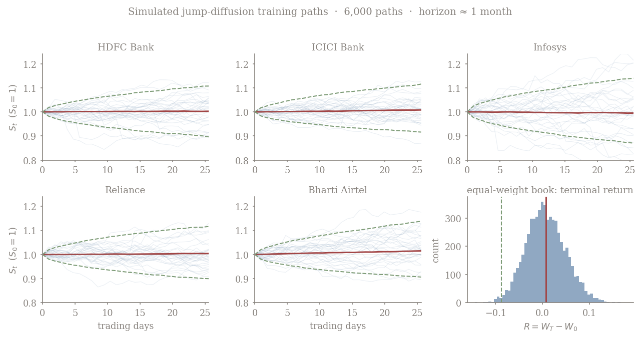
Two legs behave very differently:
The quantity scored is the terminal return \(R = W_T - W_0\), with \(W_T = W_T^{\text{stock/bond}} + \sum_j q_j\, \phi_j(S_T)\).
The paper replaces plain mean–variance with a criterion that treats the two tails asymmetrically:
\(\mathrm{ES}^{-}\) is the average of the worst \(p_1 = 1\%\) of outcomes (a large negative number; adding \(\lambda_2 \mathrm{ES}^{-}\) with \(\lambda_2 > 0\) subtracts a CVaR-style penalty proportional to how bad the left tail is), and \(\mathrm{ES}^{+}\) is the average of the best \(5\%\) (a small reward for convex upside). With \((\lambda_1, \lambda_2, \lambda_3) = (0.50,\ 0.276,\ 0.03)\) the criterion is downside-averse first and growth-seeking second.
Everything from the allocation weights through to \(U(R)\) is a single differentiable graph, evaluated on a mini-batch of simulated paths:
S (batch × 28 × 5) — the
simulated environment, no gradient;5→32→32→6 with
tanh activations, each emitting a softmax
allocation over the five stocks and the bond from the current
prices (a per-name floor keeps every stock weight positive);q · φ(S_T) added at
the end → the return vector R (length = batch);U(R) as one scalar — batch mean and variance, plus
torch.quantile and a masked mean for each shortfall
tail, all differentiable in the weights that produced R.The loss is \(-U(R)\). Adam backpropagates through the entire 27-step unrolled recursion (backprop-through-time) into all 27 networks and the option-budget logits at once — about 39k parameters, ~100 epochs, batch 4096, learning rate \(0.01\) with exponential decay. There are no labels: the option budget starts at essentially zero (logit \(-8\)) and the only training signal is "shift the controls so the simulated terminal-wealth distribution scores higher on \(U\)". It is the deep-hedging / deep-BSDE pattern — the network is the control, the SDE simulation is the environment, the loss is a distributional functional of the terminal state.
Drop \(\mathrm{ES}^{-}\) and optimise plain \(\mathbb{E}[R] - \lambda_1 \operatorname{Var}(R)\), and the cheapest way to raise the objective is to sink the whole option budget into far-out-of-the-money calls: negligible premium, large contribution to \(\mathbb{E}[R]\), and the variance penalty — nonlinear in notional — still lets a small position through. The optimum degenerates into a lottery-ticket corner solution, and the stock/bond networks drift to extremes alongside it.
The \(\lambda_2\, \mathrm{ES}^{-}\) term prices the left tail directly. In exactly the worst \(1\%\) of scenarios, an OTM premium is a dead loss and wealth is at its lowest — so \(\mathrm{ES}^{-}\) falls and the objective is penalised precisely there. That pulls the option budget back toward strikes that actually participate or protect, and forces the stock/bond networks to carry a real bond buffer. The optimum becomes an interior allocation — bond \(\approx 0.73\), five stocks \(\approx 0.016\) each, option book \(\approx 0.19\) — rather than a corner. The downside term is doing the regularisation that makes the learned weights mean something.
| metric | D-TIP (stocks + bond) | D-TIPO (+ options) |
|---|---|---|
| mean return \(\mathbb{E}[R]\) | 0.0065 | 0.076 |
| variance | 2×10⁻⁵ | 0.80 |
| lower ES (1%) | −0.0047 | −0.181 |
| upper ES (95%) | 0.015 | 3.42 |
| objective \(U\) | 0.0068 | 0.204 |
A roughly 19% option budget lifts the objective about thirty-fold, driven by the mean and the convex upside \(\mathrm{ES}^{+}\); variance and the left tail rise too, but the shortfall-aware objective still improves sharply. The static overlay is doing almost all of the work — which is also the honest reading of the next point.
A working paper of mine — an adaptive ensemble of QUBO, HRP, and CVaR optimisation with endogenous rebalancing — with a full NIFTY 50 implementation. Three allocation sleeves are switched by a hidden-Markov market-regime filter, and the book rebalances only when the regime posterior itself drifts.
Different allocation methods suit different market states: a return-seeking optimiser in calm up-markets, a diversification rule when nothing is trending, a tail-risk optimiser in stress. Rather than pick one, the framework runs all three as sleeves, infers the current market regime causally from a hidden Markov model, and lets a learned regime→sleeve map decide which sleeve holds the book — re-deciding only when the regime estimate has moved enough to matter.
Sleeve inputs \(\hat\mu_t, \hat\Sigma_t\) use a James–Stein mean and a Ledoit–Wolf covariance.
A seven-feature market-state vector drives a Gaussian HMM:
— realised volatility, 20- and 60-day index momentum, breadth (fraction of names above their 20-day average), mean pairwise correlation, drawdown, and India VIX. With \(K = 3\) states, \(P(R_t = j \mid R_{t-1} = i) = A_{ij}\) and \(X_t \mid R_t = k \sim \mathcal{N}(\mu_k, \Sigma_k)\), fit by Baum–Welch on the training window only. The posterior used everywhere is the causal filter \(p_{t,k} = P(R_t = k \mid X_{1:t})\) — a forward recursion, no smoothing, no lookahead. States are ordered by mean volatility: \(k = 0\) risk-on … \(k = K-1\) risk-off. The fitted chain is highly persistent (diagonal \(\approx 0.98\); expected regime durations \(\approx\) 74 / 43 / 59 days).
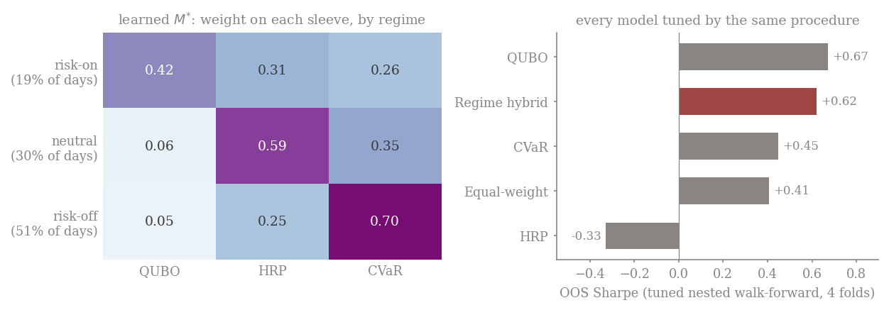
The regime score is \(a_t = M^\top p_t \in \Delta^2\) with \(M \in \mathbb{R}^{K \times 3}\) row-stochastic. \(M_0\) is a prior; the fitted \(M^\ast\) is learned per regime from sleeve returns conditioned on that regime,
shrunk toward \(M_0\); regimes with too few training days keep the \(M_0\) row. Two modes: switch (default) commits the whole book to the single sleeve \(\arg\max_j a_{t,j}\) — a regime switcher; blend holds the probability-weighted mix \(\sum_j a_{t,j}\, w_t^{j}\).
Trading is not on a calendar. From the last rebalance \(\tau\), track
and rebalance at the stopping time \(\tau_{n+1} = \inf\{ t > \tau_n : D_{\mathrm{KL},t} > \delta_p \ \text{or}\ D^{(a)}_t > \delta_a \}\), subject to a persistence check over \(m\) observations and a minimum dwell \(t - \tau \ge d_{\min}\). The holding period \(H_n = \tau_{n+1} - \tau_n\) is a random stopping time, so trading frequency tracks regime persistence — short holds in stressed blocks, long holds in calm ones.
An optional outer layer: with \(\hat\sigma_{p,t} = \sqrt{w_t^\top \Sigma_t w_t}\) (annualised), leverage \(L_t = \min(L_{\max},\ \sigma^\ast / \hat\sigma_{p,t})\) and \(w_t^{\text{final}} = L_t\, w_t\), residual in cash. The full pipeline is \(X_t \to p_t \to a_t \to w_t \to L_t \to w_t^{\text{final}}\).
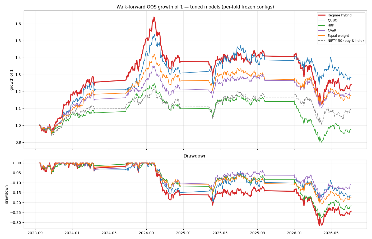
A nested walk-forward: expanding training window (\(\ge\) 3 years), 6-month OOS blocks, four outer folds. An inner train/validation split selects parameters by staged random search, and every benchmark is tuned by the same procedure against the same objective,
with transaction costs \(TC_t = c \sum_i \lvert w_{i,t} - w_{i,t^-}\rvert\) charged throughout. The benchmark hierarchy runs from single sleeves and an equal-weight null up to the full hybrid with endogenous rebalancing and volatility targeting, so each layer's marginal contribution is readable. Universe: NIFTY 50 constituents, the NIFTY index, and India VIX via Kite, 2020–2026.
| model (tuned) | Sharpe | ann. return | max DD | Calmar | score |
|---|---|---|---|---|---|
| QUBO | 0.67 | 15.3% | −10.4% | 2.68 | 0.87 |
| Regime hybrid | 0.62 | 15.0% | −13.0% | 2.81 | 0.80 |
| CVaR | 0.45 | 10.7% | −8.7% | 2.42 | 0.67 |
| Equal-weight null | 0.41 | 10.2% | −8.9% | 2.08 | 0.55 |
| HRP | −0.33 | 0.3% | −11.2% | 0.88 | −0.19 |
The honest reading: the regime hybrid did not clear the paper's own bar — §10 requires it to beat every tuned benchmark on OOS Sharpe/score. Tuned QUBO alone edged it on both. Where the hybrid did win was drawdown-adjusted return (Calmar 2.81, the best of the set): the regime machinery bought a smoother ride, not a higher risk-adjusted return. Regime-conditionally (full hybrid, OOS): risk-on \(\approx\) 15% return / 0.71 Sharpe, risk-off \(\approx\) 4.5% / \(-0.13\), and the middle "neutral" regime is where all three long-only sleeves lose money.
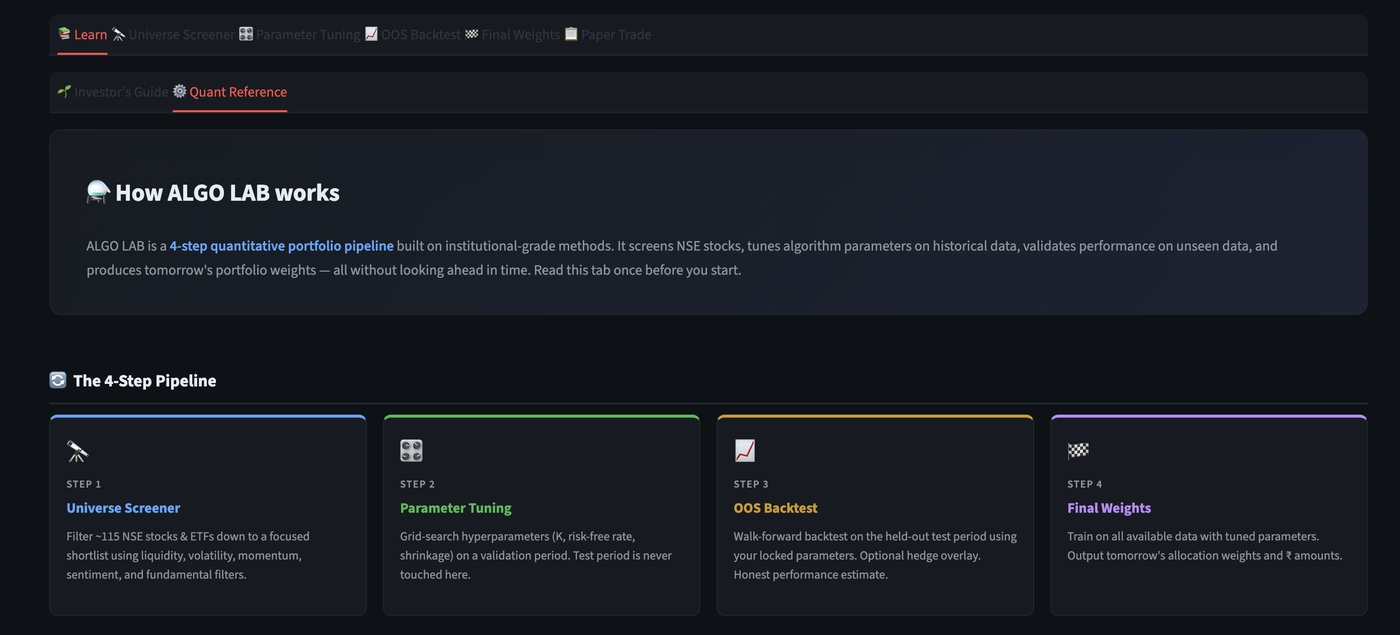
An institutional-grade quantitative portfolio platform for NSE-listed equities and ETFs, designed and built end-to-end and running live at web-production-c16cf.up.railway.app. Currently covering 111 instruments across 13 sectors.
The app turns the research pipeline — screen, construct, backtest, size — into something a user runs end-to-end in the browser, rather than a one-off notebook. It is organised as six stages; the four in the middle are the quantitative core, bookended by an onboarding Learn tab and a Paper Trade tab that tracks the chosen weights forward with no real capital at risk.
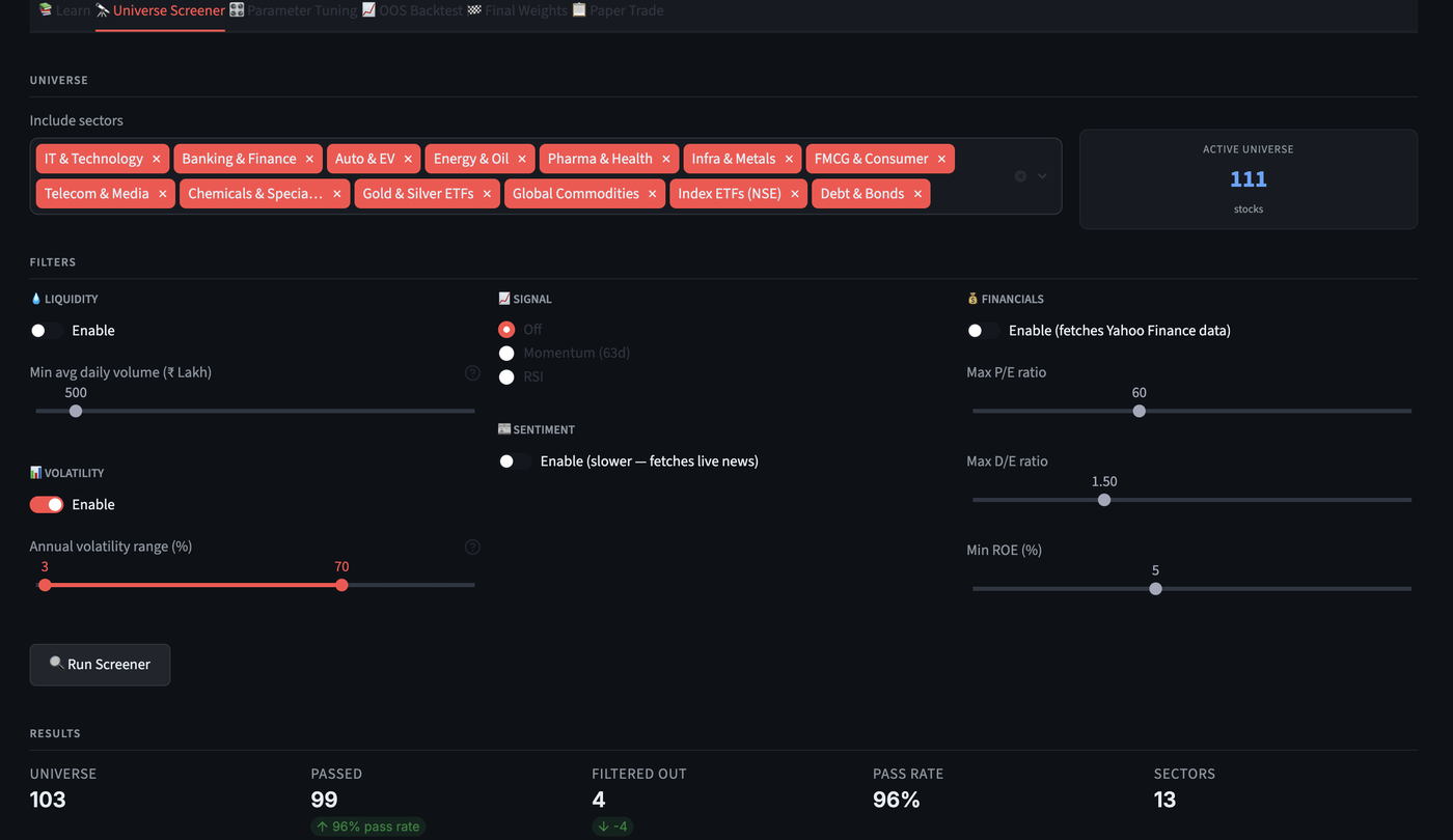
Before any optimisation runs, the instrument universe is filtered on four independent axes: liquidity (a minimum average-daily-traded-value floor), signal (off, or a 63-day momentum / RSI screen), sentiment (a slower, live news-sentiment fetch), and financials (a maximum P/E ratio against live fundamentals) — alongside always-on volatility bounds. Sector inclusion is toggled across 13 categories — from IT, banking and pharma through to gold, global commodities, and debt & bond ETFs — so the screener can be pointed at a broad multi-asset universe or narrowed to a single sleeve.
The screened universe feeds three construction methods — the same family used in the regime-hybrid working paper above: QUBO selection (quantum-inspired combinatorial optimisation via simulated annealing, plus max-Sharpe weighting on the selected support), Hierarchical Risk Parity, and Robust CVaR optimisation with an ellipsoidal robustness penalty. Inputs are stabilised with Ledoit-Wolf covariance shrinkage and James-Stein mean shrinkage, since three years of daily history is not much to estimate a covariance matrix from.
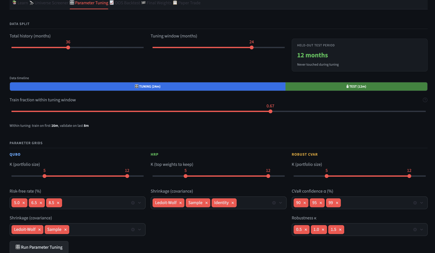
Hyperparameters are grid-searched on a strict walk-forward split: 36 months of history divide into a 24-month tuning window (trained on the first 16 months, validated on the last 8 — a 0.67 train fraction) and a 12-month held-out test period the tuner never sees. Each sleeve has its own grid — cardinality \(K \in \{5,\dots,12\}\) and covariance shrinkage for QUBO and HRP, CVaR confidence level and robustness \(\kappa\) for Robust CVaR — so the three methods are tuned on equal footing before anything is compared.
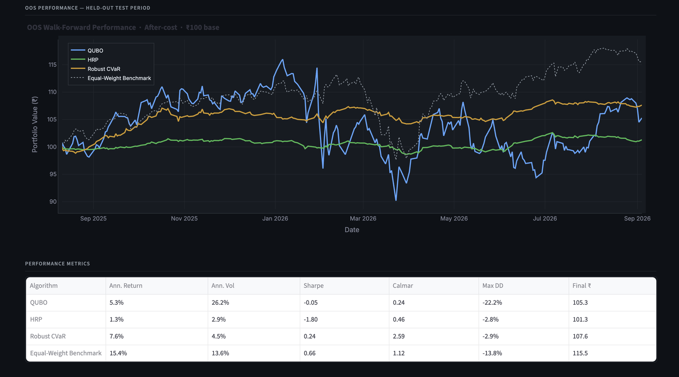
The tuned configuration is then walk-forward tested on the untouched 12 months, after transaction costs, with three optional hedge overlays available on top — Beta-Neutral (a Nifty beta hedge), Drawdown-Triggered (hysteresis-based activation), and Put-Protection (Black–Scholes-priced downside insurance). Reported plainly, because it's the honest result of one such run (Sep 2025 – Sep 2026): a naïve equal-weight book of the same universe outperformed all three optimised sleeves — 15.4% annualised return and a 0.66 Sharpe, against QUBO's 5.3% / \(-0.05\), HRP's 1.3% / \(-1.80\), and Robust CVaR's 7.6% / 0.24. Robust CVaR did hold the shallowest drawdown of the three (\(-2.9\%\) vs. QUBO's \(-22.2\%\)) — the sleeve is doing what it's built for, controlling the tail, just not out-returning a simple benchmark in this window.
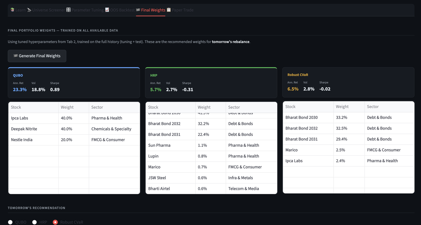
The final stage retrains each sleeve on all available data — tuning window plus test window — with the locked hyperparameters, and outputs the next rebalance's weights. In the run shown, QUBO landed on a concentrated three-name book (Ipca Labs and Deepak Nitrite at 40% each, Nestle India at 20%); HRP and Robust CVaR instead parked 80–95% of the book in Bharat Bond government-bond ETFs, with only a thin residual equity sleeve — a defensive tilt that is exactly what those two objectives are supposed to produce when the optimiser sees little reward for taking equity risk.